Regression discontinuity with sci-kit learn models

from sklearn.gaussian_process import GaussianProcessRegressor
from sklearn.gaussian_process.kernels import ExpSineSquared, WhiteKernel
from sklearn.linear_model import LinearRegression

import causalpy as cp

%config InlineBackend.figure_format = 'retina'

Load data

data = cp.load_data("rd")
data.head()

	x	y	treated
0	-0.932739	-0.091919	False
1	-0.930778	-0.382663	False
2	-0.929110	-0.181786	False
3	-0.907419	-0.288245	False
4	-0.882469	-0.420811	False

Linear, main-effects model

result = cp.RegressionDiscontinuity(
    data,
    formula="y ~ 1 + x + treated",
    model=LinearRegression(),
    treatment_threshold=0.5,
)

fig, ax = result.plot()

/Users/benjamv/opt/mambaforge/envs/CausalPy/lib/python3.11/site-packages/IPython/core/pylabtools.py:77: DeprecationWarning: backend2gui is deprecated since IPython 8.24, backends are managed in matplotlib and can be externally registered.
  warnings.warn(
/Users/benjamv/opt/mambaforge/envs/CausalPy/lib/python3.11/site-packages/matplotlib_inline/config.py:68: DeprecationWarning: InlineBackend._figure_format_changed is deprecated in traitlets 4.1: use @observe and @unobserve instead.
  def _figure_format_changed(self, name, old, new):
/Users/benjamv/opt/mambaforge/envs/CausalPy/lib/python3.11/site-packages/IPython/core/pylabtools.py:77: DeprecationWarning: backend2gui is deprecated since IPython 8.24, backends are managed in matplotlib and can be externally registered.
  warnings.warn(
/Users/benjamv/opt/mambaforge/envs/CausalPy/lib/python3.11/site-packages/IPython/core/pylabtools.py:77: DeprecationWarning: backend2gui is deprecated since IPython 8.24, backends are managed in matplotlib and can be externally registered.
  warnings.warn(

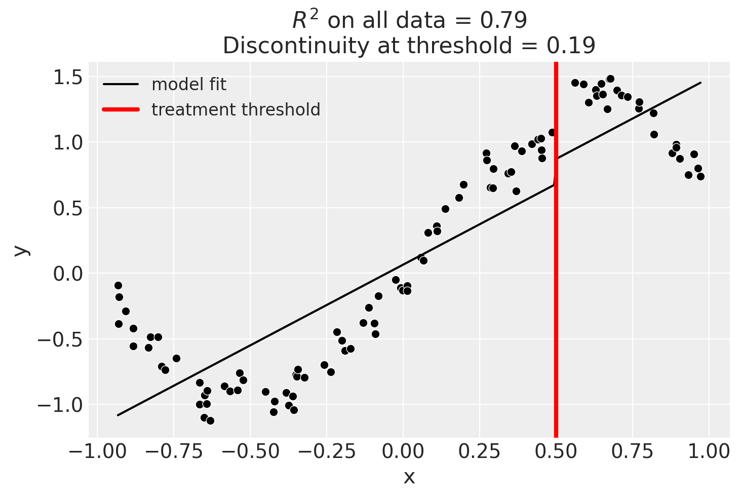
result.summary(round_to=3)

Difference in Differences experiment
Formula: y ~ 1 + x + treated
Running variable: x
Threshold on running variable: 0.5

Results:
Discontinuity at threshold = 0.19


Model coefficients:
  Intercept      	         0
  treated[T.True]	      0.19
  x              	      1.23

Linear, main-effects, and interaction model

result = cp.RegressionDiscontinuity(
    data,
    formula="y ~ 1 + x + treated + x:treated",
    model=LinearRegression(),
    treatment_threshold=0.5,
)

result.plot();

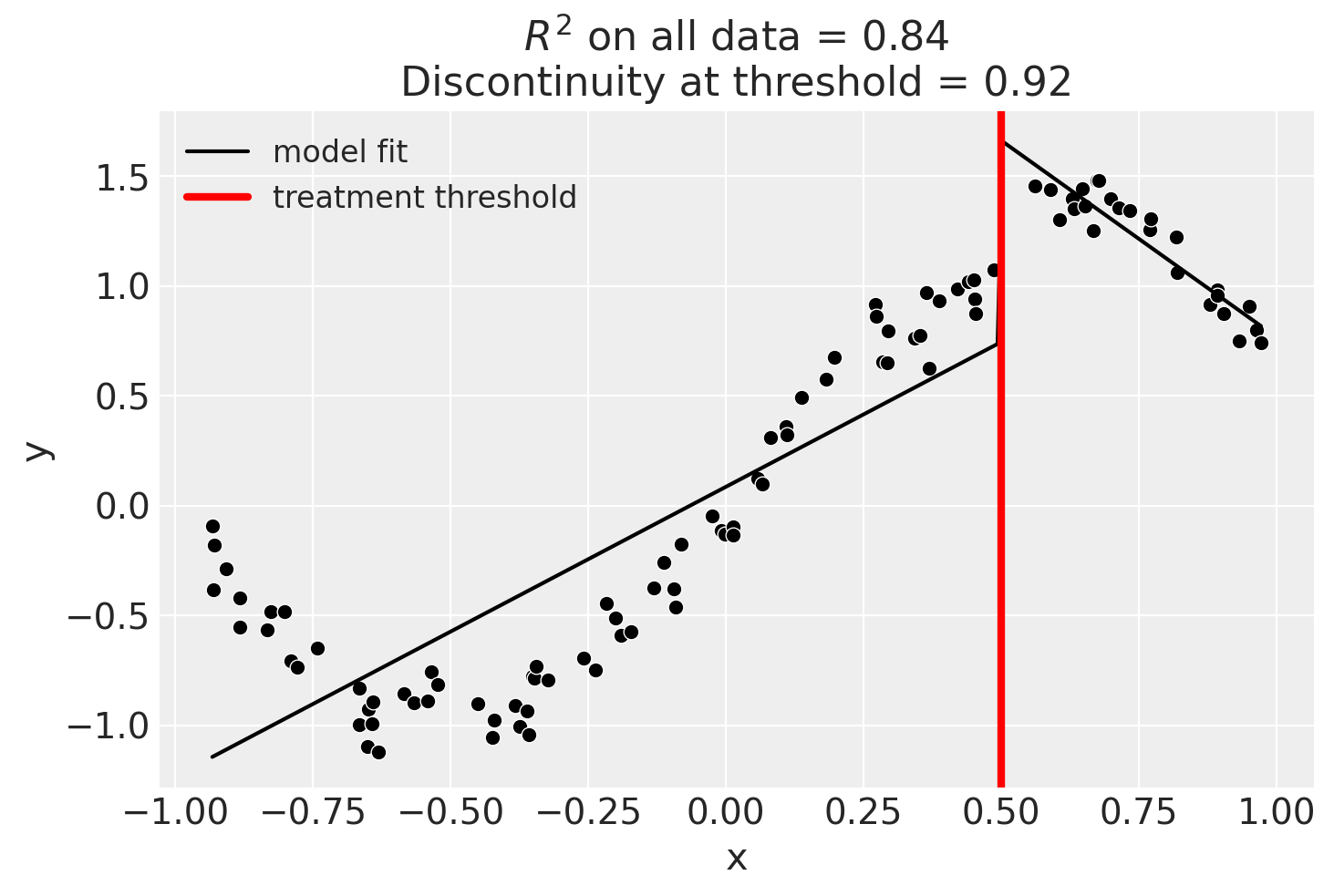
Though we can see that this does not give a good fit of the data almost certainly overestimates the discontinuity at threshold.

result.summary(round_to=3)

Difference in Differences experiment
Formula: y ~ 1 + x + treated + x:treated
Running variable: x
Threshold on running variable: 0.5

Results:
Discontinuity at threshold = 0.92


Model coefficients:
  Intercept        	         0
  treated[T.True]  	      2.47
  x                	      1.32
  x:treated[T.True]	     -3.11

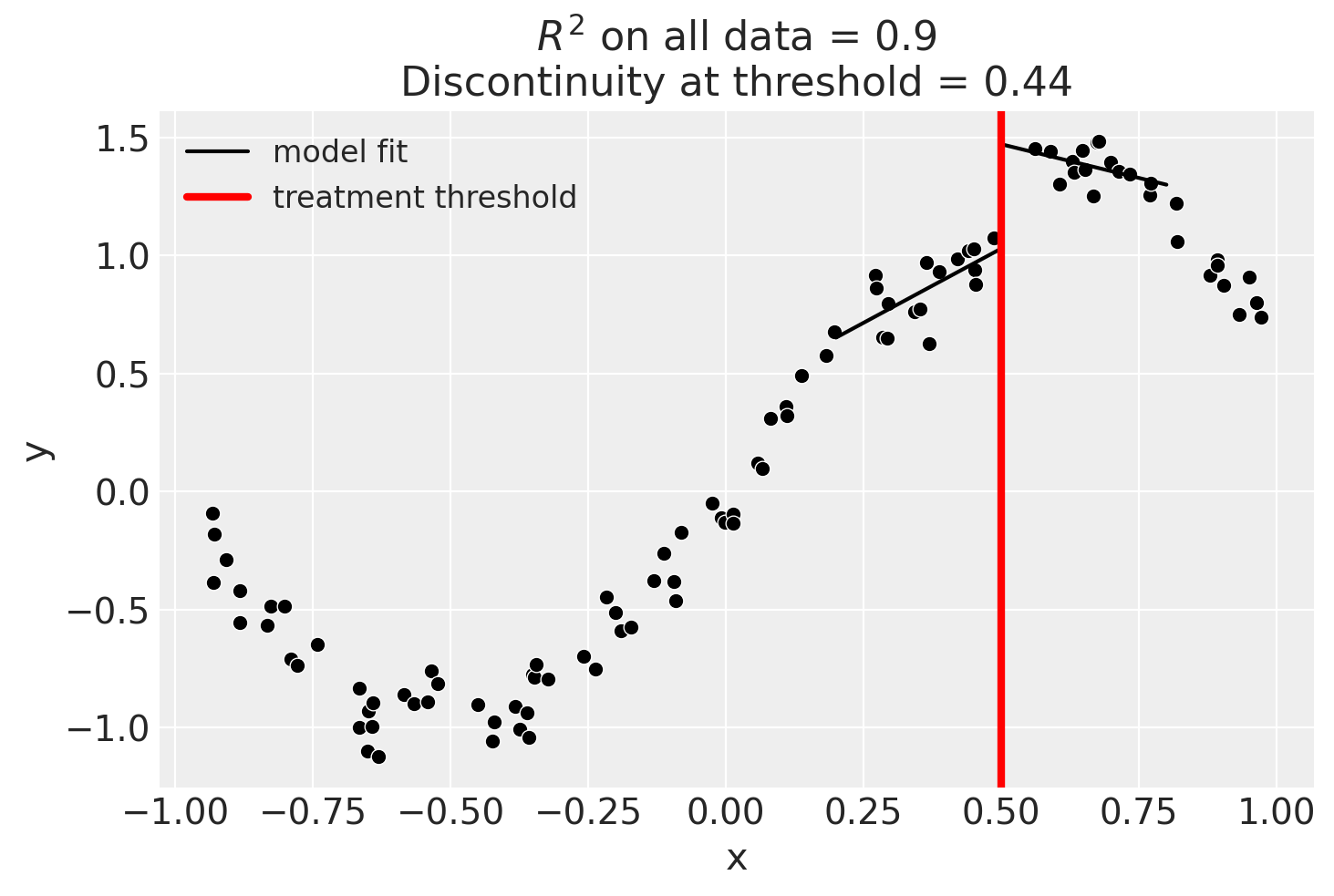
Using a bandwidth

One way how we could deal with this is to use the bandwidth kwarg. This will only fit the model to data within a certain bandwidth of the threshold. If \(x\) is the running variable, then the model will only be fitted to data where \(threshold - bandwidth \le x \le threshold + bandwidth\).

result = cp.RegressionDiscontinuity(
    data,
    formula="y ~ 1 + x + treated + x:treated",
    model=LinearRegression(),
    treatment_threshold=0.5,
    bandwidth=0.3,
)

result.plot();

We could even go crazy and just fit intercepts for the data close to the threshold. But clearly this will involve more estimation error as we are using less data.

result = cp.RegressionDiscontinuity(
    data,
    formula="y ~ 1 + treated",
    model=LinearRegression(),
    treatment_threshold=0.5,
    bandwidth=0.3,
)

result.plot();

Using Gaussian Processes

Now we will demonstrate how to use a scikit-learn model.

kernel = 1.0 * ExpSineSquared(1.0, 5.0) + WhiteKernel(1e-1)
result = cp.RegressionDiscontinuity(
    data,
    formula="y ~ 1 + x + treated",
    model=GaussianProcessRegressor(kernel=kernel),
    treatment_threshold=0.5,
)

fig, ax = result.plot()

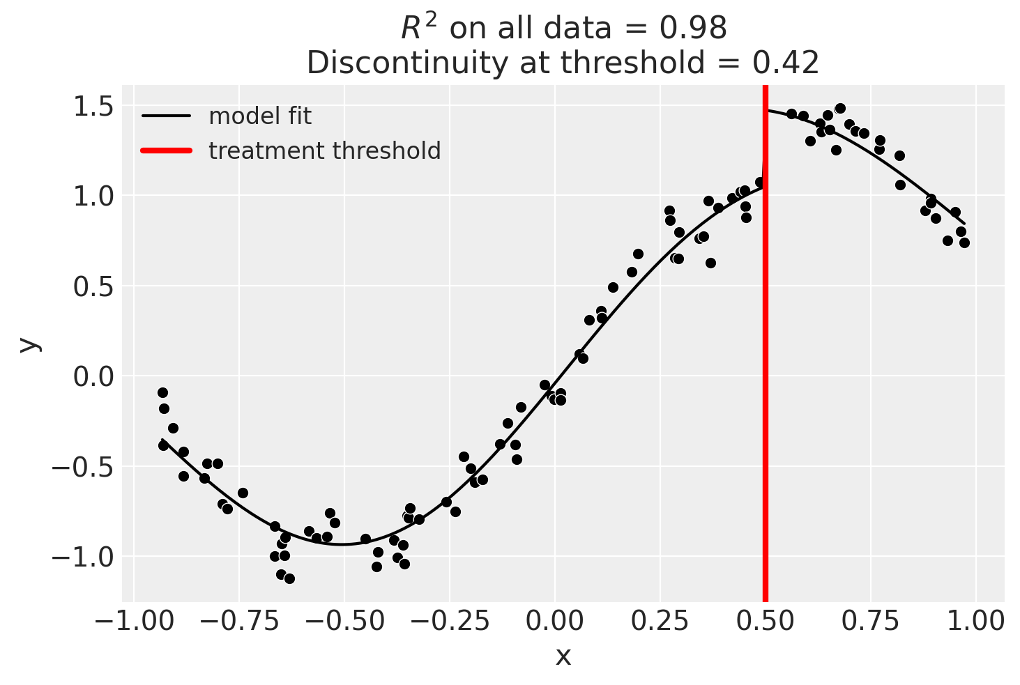
Using basis splines

result = cp.RegressionDiscontinuity(
    data,
    formula="y ~ 1 + bs(x, df=6) + treated",
    model=LinearRegression(),
    treatment_threshold=0.5,
)

fig, ax = result.plot()

result.summary(round_to=3)

Difference in Differences experiment
Formula: y ~ 1 + bs(x, df=6) + treated
Running variable: x
Threshold on running variable: 0.5

Results:
Discontinuity at threshold = 0.41


Model coefficients:
  Intercept      	         0
  treated[T.True]	     0.407
  bs(x, df=6)[0] 	    -0.594
  bs(x, df=6)[1] 	     -1.07
  bs(x, df=6)[2] 	     0.278
  bs(x, df=6)[3] 	      1.65
  bs(x, df=6)[4] 	      1.03
  bs(x, df=6)[5] 	     0.567